Classifying MNIST as 1D Signals
The MNIST dataset of hand-written digits is ubiquitous in image classification, the de facto “hello world” of 2D CNNs. It’s also famously easy – a decent model can achieve 98% accuracy with a few minutes of training.
To keep things interesting, let’s try dropping a dimension. Can we make MNIST fun again by treating it as a 1D signal classification problem?
Images to Signals
There are a lot of ways to convert a 2D image to a 1D signal. The simplest approach is to just ravel a 28x28 image into 784 sequential pixels, discarding 2D location data but retaining individual pixels values. I want to try something more interesting: an aggregation in polar space.
Images are usually represented in Cartesian (x, y) coordinates, but with a little math they can be reprojected into polar coordinates that represent the angle and distance of each pixel from an origin point.
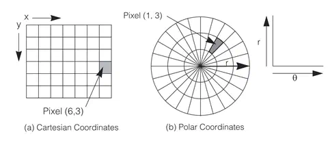
Cartesian to polar coordinate conversion, via Cognex.
Polar transformations are useful for coregistering images because rotations in Cartesian space appear as translations in polar space, but for converting images to signals they have another interesting property: summing pixels along the radial axis provides a profile of how each digit is radially distributed around the image center:
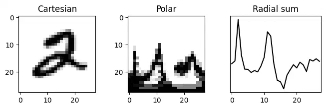
An MNIST digit in Cartesian and polar coordinates, and its radial distribution around the image center.
Polar projections are hard to wrap your head around, so another way to think about aggregating in the radial dimension is to imagine casting a ray outwards from the image center in Cartesian coordinates. If you rotate the ray 360 degrees and count the pixels at each angle1, you’ll get the same radial profile we saw above:
Repeating this projection-aggregation process over a few dozen MNIST digits starts to reveal common patterns in their radial distributions, which is what we’ll leverage to build a signal classifier.
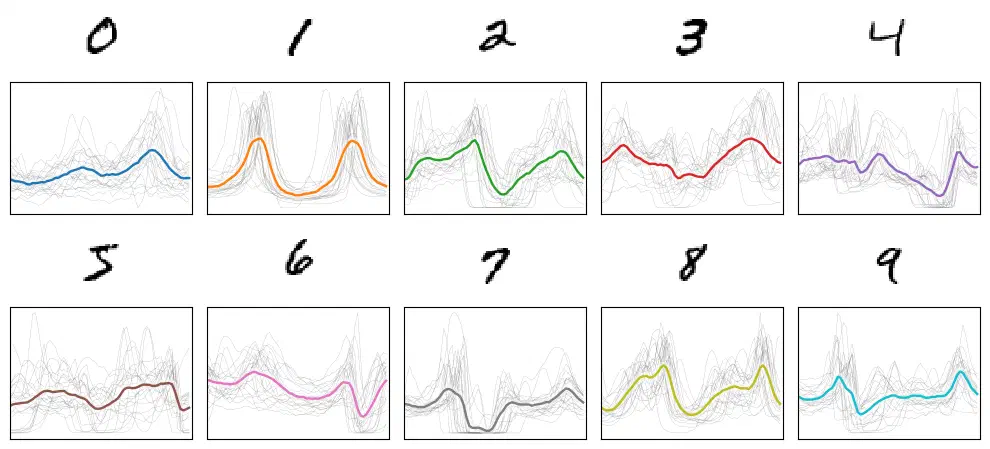
Mean radial sum signals for a sample of each MNIST digit.
The Classifier
Traditional ML approaches to signal classification start with extracting salient features using techniques like Fourier transforms and wavelet decomposition, but we can offload a lot of that complexity onto the model by using a 1D CNN that will identify its own features via convolution.
I built a pretty standard 1D CNN in Pytorch with the modification of 1) large kernel sizes since we’re more interested in low-frequency patterns than high-frequency detail, and 2) circular padding to allow convolutions to wrap around the array edges, since the radial distributions are inherently cyclical.
Training for 10 epochs gives a very respectable 95.4% accuracy. It’s not quite the ~98% accuracy you can get with a 2D CNN, but it’s better than I was expecting after aggregating away an entire dimension.
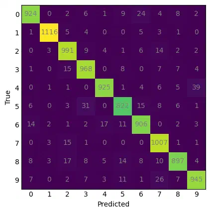
Confusion matrix of predicted and observed digits from the 1D CNN.
You can find the full code for this project on Github.
The angular resolution of the radial sum, i.e. the number of samples in the 1D array, can be adjusted by resampling the input image. ↩︎