Measuring Dead Trees from Aerial Photos
My day job involves a lot of time spent looking at NAIP aerial imagery of burned forests. The scene below is pretty common: large swaths of high severity fire leave behind hectares of standing dead snags. While the trees themselves can be hard to make out after needles drop, the distinctive shadows that they cast are a dead giveaway.
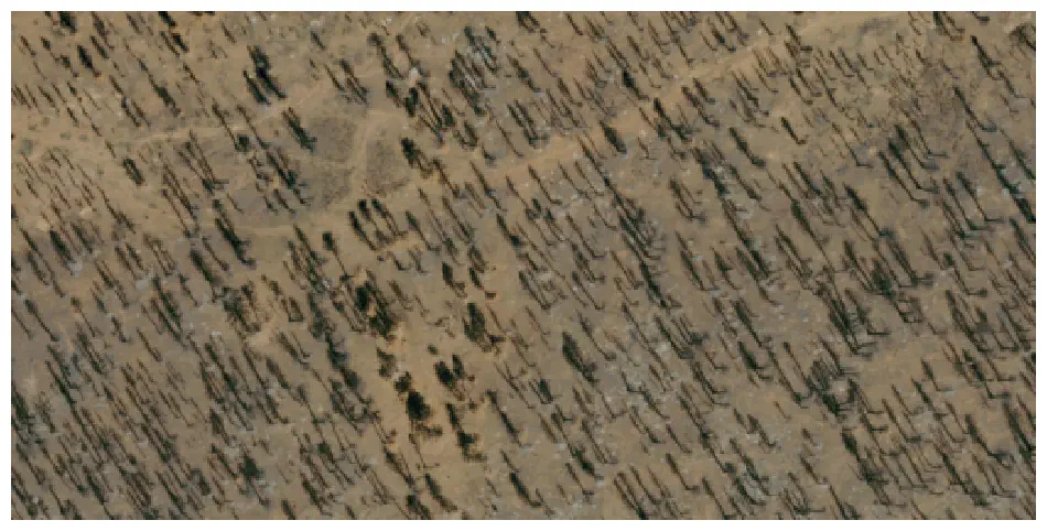
Diagonal shadows cast by standing dead snags in a burned forest.
These snag fields are ecologically important as early seral habitat, but they also pose a hazard to humans working in and around them. In either case, knowing where the tall snags are is valuable.
While LiDAR is the de-facto approach for accurately measuring the height of live trees, dead trees pose a challenge. With no canopy of healthy leaves to reflect laser pulses, snags present a much smaller target; even with high point density, it’s easy to miss the true top and underestimate height.
What if we could indirectly measure snag height with freely available aerial imagery by measuring their shadows?
The idea
The concept is simple: a vertical object casts a shadow of length $ℓ$ as a function of the object’s height $h$ and the angle of the light source $α$. On a slope, we’ll also need to account for the change in elevation $dz$ across the length of the shadow. The full equation is:
$$ h = \tan(α) \times ℓ + dz $$
If we can measure $ℓ$ from the photo, calculate $α$ when the photo was taken, and extract $dz$ from a DEM, we’ll have everything needed to solve for snag height $h$. That’s the plan, anyways.
Seamlines and solar elevation
Alongside the state-wide mosaics that they publish every couple years, NAIP releases a dataset of seamline polygons that describe the local approximate time that each area was photographed. With a time and location, a package like pvlib can calculate the corresponding solar position.
For example, here’s the solar elevation (angle above the horizon) for NAIP acquisitions over Oregon in 20111.
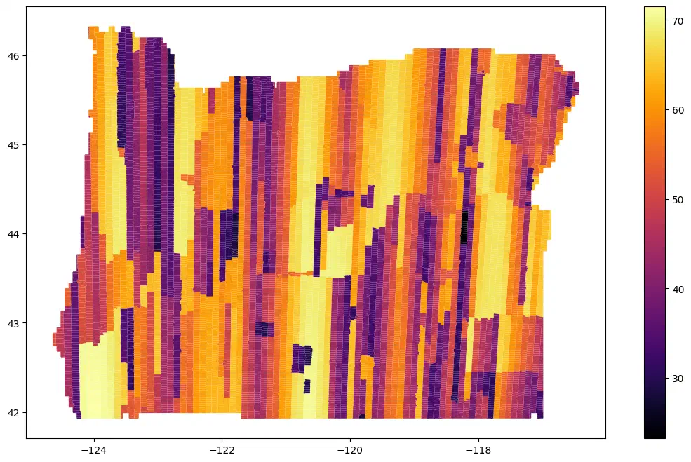
Oregon 2011 NAIP seamlines color-coded by the solar elevation when each seam was acquired.
That solves the first unknown in the snag height equation; for any given snag we can calculate the solar elevation and azimuth at the corresponding seamline. Now we just need to know the length of shadow that each tree casts.
Measuring shadows
Extracting straight line features like tree shadows from an image full of noise – soil, rocks, and leaves, to name a few – is a classic computer vision problem. I experimented with off-the-shelf line detection methods like Hough transforms and line segment detection, but the results were inconsistent at best2. I ultimately landed on simple adaptive thresholding with some post-processing.
Thresholding the NAIP imagery’s shadow index – the inverted product of the RGB3 bands – produced a binary mask that separated shadow from non-shadow reasonably well.
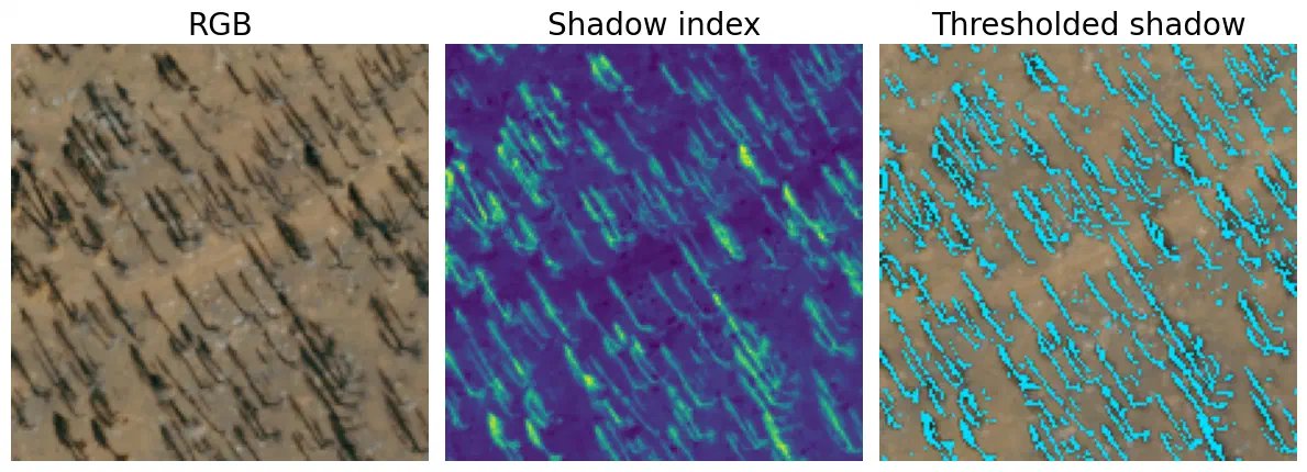
If you look closely at the segmented shadows, you’ll see some leaning snags (likely due to the photo being slightly off-nadir - more on that later) are being included in addition to the real tree shadows. To accurately measure tree height, each shadow needs to be distinct, so those intersecting off-angle shadows are a problem.
This is where our a priori knowledge about sun position comes in handy. We know the solar azimuth and the corresponding angle of the true snag shadows (accounting for meridean convergence in the image projection4). If we run a convolution kernel designed to match that expected shadow line over the segmented shadows, it should highlight lines at or near that angle while suppressing spurious angles.
Masking the thresholded shadows with their convolution generates a much cleaner final shadow mask.
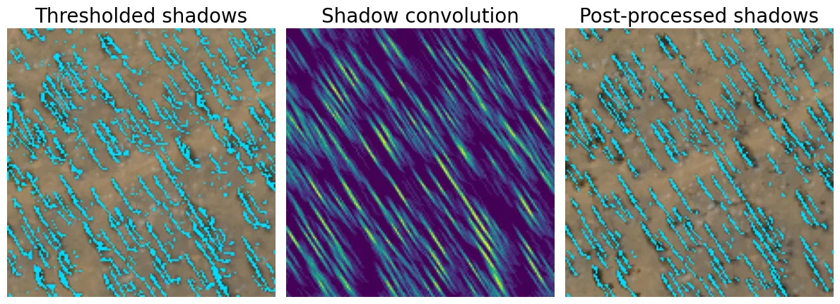
The final step to estimating shadow lengths is to iterate over each set of connected pixels, calculating the straight-line distance between their extreme coordinates.
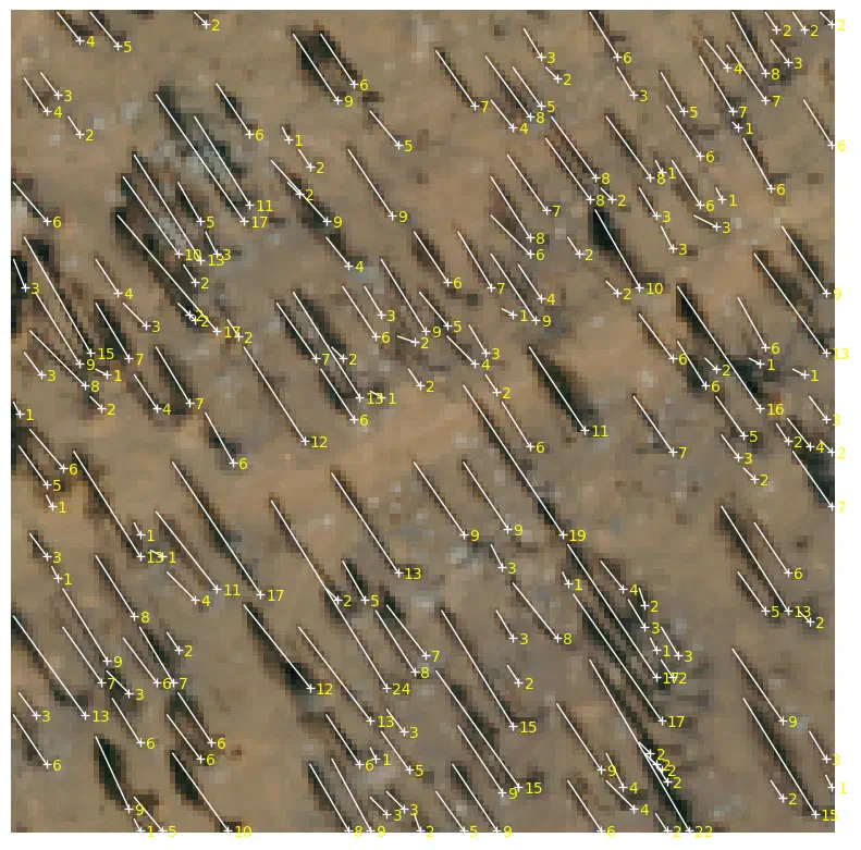
Detected tree shadows and their lengths in meters.
Simulated snags
Finally, we can loop over each measured tree shadow, calculate the change in elevation $dz$ between its ends from a DEM, and plug everything into the snag height equation.
That yields 204 individual snags within the pictured 8100m2 area (252 snags per hectare) with a mean height of 15m and a max height of 61m. I don’t have plot data to validate height estimates, but by reconstructing the snags in 3D and simulating shadows from the solar position, we should get a good visual check of how well the simulated shadows match those seen in the NAIP imagery.
You can see the results for yourself in the interactive demo below (click and drag to rotate, click the button to see how well the simulated shadows overlap the imagery).
Looks pretty good to me.
Does it generalize?
It’s hard to make any strong claims without quantitative validation, but it seems like using computer vision to estimate snag heights from shadows can be a viable alternative to LiDAR and field work in the right circumstances. The challenge, as is often the case with computer vision, is generalizability.
Once you start looking at denser stands, leaning snags, lower burn severity, and off-nadir imagery, this approach is going to break down pretty quickly, and you’d probably be better off scraping together a dataset and training a CNN. But for a quick estimate under ideal conditions, it’s hard to beat the simplicity of classic computer vision.
If you’ve ever struggled with inconsistent lighting in NAIP scenes, that solar elevation map should explain why - sun angle can change by 50 degrees between neighboring pixels. ↩︎
The Hough transform did well with some trees, but had a habit of splitting single long shadows into many short ones perpendicular to the shadow angle. There might be some combination of parameters that would perform well, but I never found it. The line segment detector tended to identify two lines on either side of each shadow, rather than the shadow itself. ↩︎
I experimented with other band combinations and ratios. The RGB shadow index provided the best contrast. ↩︎
North in the image projection isn’t necessarily the true north that solar azimuth is measured from, which is why we need to account for meridean convergence. I used
pyproj.Proj.get_factorsto calculate the angle offset. ↩︎