Terrain Algorithms on the GPU with Taichi

A few years back, I explored some common terrain algorithms like slope, aspect, and hillshading by implementing them from scratch in Python. I was more interested in keeping things simple and understandable than fast, so I used a lot of nested Python loops and serial pixel-level calculations on the CPU, creating some truly sluggish code.

After recently re-watching my way through Sebastian Lague’s fantastic Coding Adventures series on Youtube, I got inspired to revisit those algorithms with a compute shader to see how fast we can get them running on the GPU. And while I’m at it, let’s also look at some other hillshading variants like multi-directional and Igor hillshading.

Of course, Python can’t write GPU shaders on its own, so the first thing we’ll need is a GPU-compatible language.

Talking to the GPU

There are a lot of ways to write Python-like code for the GPU these days, but I’ve been looking for an excuse to try out Taichi. As a Python subset, it lacks some of the flexibility of general-purpose GPU-focused programming languages like Bend or Mojo, but the ability to interoperate with other Python code without learning any new syntax or tooling is pretty appealing¹, so that’s what I’ll be using.

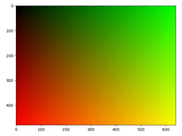
Most of the magic in Taichi comes from the ti.kernel decorator, which can convert a typed Python function into a CUDA kernel, automatically parallelizing loops across GPU threads. For example, we can write a basic shader that takes the X and Y coordinates of a Numpy array and maps them to brightness in the green and red channels:

import taichi as ti
import numpy as np

@ti.kernel
def frag(uv: ti.types.ndarray()):
    """
    A fragment shader that sets green and red channels to normalized x, y coordinates.
    """
    for y, x, _ in uv:
        uv[y, x, 0] = y / uv.shape[0]
        uv[y, x, 1] = x / uv.shape[1]

ti.init(arch=ti.cuda)
buffer = np.zeros((480, 640, 3))
frag(buffer)

When we call frag with a Numpy array, Taichi JIT compiles the function into a CUDA kernel and parallelizes the operation across every pixel in the buffer, mutating them in-place to give us this lovely output:

With that rudimentary understanding of Taichi, let’s see if we can re-implement our terrain algorithms for the GPU.

Terrain Kernels

Slope

There’s more detail in the original blog post, but just to quickly recap, slope and aspect are calculated by looking at the rate of elevation change around a point. We’ll eventually write kernels to calculate slope and aspect at every cell on a digital elevation model (DEM) in parallel, but first let’s just write a function to calculate the east-west and north-south gradients, $\frac{dz}{dx}$ and $\frac{dz}{dy}$ respectively, at a single location. To do that, we’ll simply get the difference between neighboring cells on each axis from the DEM and normalize that by the number of cells and the distance between them, ${dx}$.

@ti.func
def calculate_gradients(dem: ti.types.ndarray(), x: int, y: int, dx: float):
    """
    Calculate EW and NS gradients at index (x, y) on a DEM using the Horn algorithm.
    """
    # Cardinal neighbors
    zw = dem[y, x-1]
    ze = dem[y, x+1]
    zs = dem[y+1, x]
    zn = dem[y-1, x]

    # Diagonal neighbors
    znw = dem[y-1, x-1]
    zsw = dem[y+1, x-1]
    zne = dem[y-1, x+1]
    zse = dem[y+1, x+1]

    # East-west gradient
    dz_dx = ((zne + zse + 2 * ze) - (znw + zsw + 2 * zw)) / 8 / dx

    # North-south gradient
    dz_dy = ((zsw + zse + 2 * zs) - (znw + zne + 2 * zn)) / 8 / dx

    return dz_dx, dz_dy

We’re using a new decorator ti.func here, which just means that we can call this compiled function on the GPU from within our kernel.

With the gradients calculated, we can now derive slope with a little trigonometry using the equation below. We’ll need to calculate this a few times, so I wrote a quick helper function for reusability:

$$ slope _{radians} = \arctan \sqrt {\frac{dz}{dx}^2 + \frac{dz}{dy}^2} $$

import taichi.math as tm

@ti.func
def gradients_to_slope(dz_dx: float, dz_dy: float) -> float:
    """Convert gradients to slope in radians."""
    return tm.atan2((dz_dx ** 2 + dz_dy ** 2) ** 0.5, 1.0)

Now we can put these pieces together to write our first real GPU kernel, which will take a DEM array containing elevation values, a buffer array into which we can write results, and the cell spacing ${dx}$, and calculate slope for every pixel in the buffer.

@ti.kernel
def calculate_slope(dem: ti.types.ndarray(), buf: ti.types.ndarray(), dx: float):
    """Calculate slope in degrees from a DEM."""
    H, W = dem.shape
    
    for y, x in buf:
        # Bounds check to avoid accessing invalid memory
        if x == 0 or y == 0 or x == W - 1 or y == H - 1:
            continue
        
        gradients = calculate_gradients(dem, x, y, dx)
        slope = gradients_to_slope(*gradients)
        buf[y, x] = tm.degrees(slope)

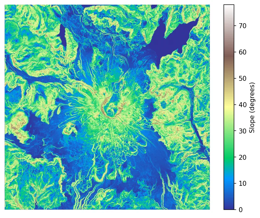
I loaded a 10m DEM with 2048 x 2048 pixels around Mt. St. Helens, passed it to kernel, and a split second later, we’ve got a slope map.

That was definitely fast, but let’s finish writing some more kernels before diving too deep into performance.

Aspect

To calculate aspect, we’ll write another helper function for the equation below, with some added terms to convert from Euclidean angles measured counter-clockwise from East, to compass bearings measured clockwise from North:

$$ aspect = \arctan2 \left( \frac{dz}{dy}, -\frac{dz}{dx} \right) $$

@ti.func
def gradients_to_aspect(dz_dx: float, dz_dy: float) -> float:
    """Convert gradients to aspect in radians, clockwise from North."""
    aspect = tm.pi / 2 - tm.atan2(dz_dy, -dz_dx)
    if aspect < 0:
        aspect += 2 * tm.pi    
    return aspect

The aspect shader follows the same pattern as the slope shader; all we need to swap is the helper function:

@ti.kernel
def calculate_aspect(dem: ti.types.ndarray(), buf: ti.types.ndarray(), dx: float):
    """Calculate aspect in degrees from a DEM."""
    H, W = dem.shape
    
    for y, x in buf:
        if x == 0 or y == 0 or x == W - 1 or y == H - 1:
            continue

        gradients = calculate_gradients(dem, x, y, dx)
        aspect = gradients_to_aspect(*gradients)
        buf[y, x] = tm.degrees(aspect)

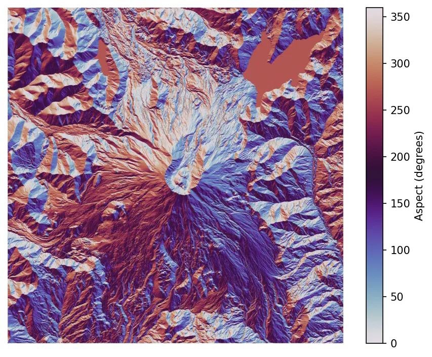
And here’s our aspect map:

Hillshading

With slope and aspect done, we can combine them to get classic hillshading at a given solar zenith and azimuth using the formula:

$$ hillshade = \cos(zenith) * \cos(slope) + \sin(zenith) * \sin(slope) * \cos(azimuth - aspect) $$

Converting that into a Taichi kernel gives us the code below.

@ti.kernel
def calculate_hillshade(dem: ti.types.ndarray(), buf: ti.types.ndarray(), dx: float, azimuth: float, altitude: float):
    H, W = dem.shape
    for y, x in buf:
        if x == 0 or y == 0 or x == W - 1 or y == H - 1:
            continue

        gradients = calculate_gradients(dem, x, y, dx)
        aspect = gradients_to_aspect(*gradients)
        slope = gradients_to_slope(*gradients)

        zenith = tm.radians(90 - altitude)
        azim = tm.radians(azimuth)

        hs = tm.cos(zenith) * tm.cos(slope) + tm.sin(zenith) * tm.sin(slope) * tm.cos(azim - aspect)
        buf[y, x] = tm.clamp(hs, 0.0, 1.0)

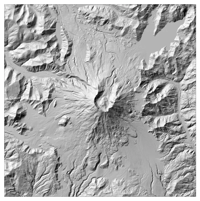
That looks like classic hillshading – let’s try some different variants next.

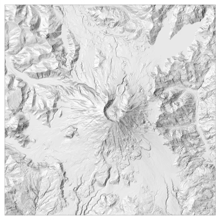
Multi-directional Hillshading

As the name suggests, multi-directional hillshading is just like normal hillshading, but computed from a few different azimuths with different weights applied. We can loop over each azimuth using ti.static for loop unrolling, and accumulate the weighted hillshade into the buffer:

@ti.kernel
def calculate_multidirectional_hillshade(dem: ti.types.ndarray(), buf: ti.types.ndarray(), dx: float, altitude: float):
    """
    Calculate a multi-directional hillshade from a DEM.

    See https://pubs.usgs.gov/of/1992/of92-422/of92-422.pdf
    """
    H, W = dem.shape
    for y, x in buf:
        if x == 0 or y == 0 or x == W - 1 or y == H - 1:
            continue

        gradients = calculate_gradients(dem, x, y, dx)
        aspect = gradients_to_aspect(*gradients)
        slope = gradients_to_slope(*gradients)
        zenith = tm.radians(90 - altitude)

        cumulative_hs = 0.0
        for azimuth in ti.static((225, 270, 315, 360)):
            azim = tm.radians(azimuth)
            weight = tm.sin(aspect - azim) ** 2
            hs = tm.cos(zenith) * tm.cos(slope) + tm.sin(zenith) * tm.sin(slope) * tm.cos(azim - aspect)
            cumulative_hs += hs * weight

        buf[y, x] = tm.clamp(cumulative_hs / 2.0, 0, 1.0)

Igor Hillshading

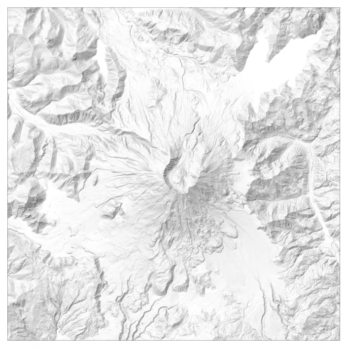
Originally developed for Maperative, Igor hillshading is another spin on the algorithm that calculates shadow strength based on terrain steepness and the difference between the terrain aspect and the solar azimuth. This requires a couple more helper functions, but otherwise looks a lot like the other kernels we’ve already implemented.

@ti.func
def normalize_angle(angle: float, normalizer: float) -> float:
    angle = angle % normalizer
    if angle < 0:
        angle = normalizer + angle
    return angle


@ti.func
def difference_between_angles(a: float, b: float, normalizer: float) -> float:
    diff = normalize_angle(a, normalizer) - normalize_angle(b, normalizer)
    diff = abs(diff)
    if diff > normalizer / 2:
        diff = normalizer - diff
    return diff 


@ti.kernel
def calculate_igor_hillshade(dem: ti.types.ndarray(), buf: ti.types.ndarray(), dx: float, azimuth: float):
    """
    Calculate an Igor hillshade from a DEM.

    See https://github.com/OSGeo/gdal/issues/1330
    """
    H, W = dem.shape
    for y, x in buf:
        if x == 0 or y == 0 or x == W - 1 or y == H - 1:
            continue

        dz_dx, dz_dy = calculate_gradients(dem, x, y, dx)
        # The Igor algorithm uses raw aspect rather than aspect clockwise from North
        aspect = tm.atan2(dz_dy, -dz_dx)
        slope = gradients_to_slope(dz_dx, dz_dy)

        aspect_diff = difference_between_angles(aspect, tm.pi * 3/2 - tm.radians(azimuth), tm.pi * 2)
        slope_strength = tm.clamp(slope, 0, tm.pi / 2) / (tm.pi / 2)
        aspect_strength = 1 - aspect_diff / tm.pi
        shadowness = slope_strength * aspect_strength

        buf[y, x] = tm.clamp(1 - shadowness, 0.0, 1.0)

We’ve got a good selection of kernels now that all look reassuringly correct, and they certainly feel fast, but just how fast are they really? Time for some benchmarking.

Performance

Just to get a baseline with an unoptimized, naive implementation of classic hillshading, I ran my original, serial Python code over the 2048 x 2048 DEM. This was never meant to be efficient, and it shows; the hillshade takes 79 seconds to compute. Yikes.

For a more fair comparison to how you’d typically implement this kind of algorithm in Python, I rewrote it using vectorized Numpy and Scipy. Offloading most of the expensive looping to compiled C code reduced the total time to just 482 milliseconds. This is why we don’t use Python loops.

What about Taichi? On the massively parallel, blazingly fast GPU, our hillshade computation takes… 687 milliseconds, a bit slower than Numpy on the CPU. That’s a little anti-climactic, but I think what we’re seeing here is the expected overhead of JIT compiling our kernel and moving data back and forth between the CPU and GPU.

That overhead should matter a lot less with larger datasets or repeated computations using the same kernel, and that seems to check out in practice. Computing a much larger hillshade of 16,384 x 16,384 pixels runs in 11.8 seconds on the GPU, about 4x faster than Numpy. Things would look even better if our DEM stayed on the GPU for multiple computations – even with this massive input array, the profiler says that the kernel itself only takes 32 milliseconds to compute, so it seems the vast majority of the time is still being spent on compiling kernels and moving data around.

Conclusion

It wasn’t quite the guaranteed speed-up I was hoping for, but moving these algorithms to the GPU was surprisingly easy with Taichi, and undeniably fast – potentially much faster than calculating them on the CPU, under the perfect conditions. I’m also quite new to Taichi, so there are probably plenty of optimizations to be made; I really need to spend some time reading through their performance tuning tips, for a start.

While Taichi’s simplicity made it very easy to dive into without knowing much about GPU programming or CUDA, I did frequently find myself wondering what exactly it’s doing behind the scenes. For example, most GPU APIs that I’ve seen use explicit operations to move data from the CPU to the GPU and synchronize results. Having Taichi handle that implicitly is convenient, but did make me question whether I’m shooting myself in the foot with unnecessary or inefficient transfers. Maybe it’s smart enough to prevent me from making silly mistakes, but I’d personally feel more comfortable with something a little lower-level.