Terrain Algorithms from Scratch

There are plenty of tools to calculate slope, aspect, and hillshading from elevation data, but if you've ever been curious about how they're calculated, this post goes through the process of implementing those algorithms from scratch in Python using just Numpy.

Elevation Data

Terrain algorithms won't do much good without elevation data to apply them to, so the first thing we'll do is to grab some of that. Specifically, we'll download a digital elevation model (DEM) over Mount St. Helens from Microsoft Planetary Computer. Using STAC (via pystac-client) will allow us to quickly find the asset we need, and the stackstac package will make it easy to download and clip it into a 2D Numpy array.

python
Copy
from pystac_client import Client
import planetary_computer as pc
import stackstac


# Load the Planetary Computer catalog
catalog = Client.open("https://planetarycomputer.microsoft.com/api/stac/v1")

# Define the bounding box around Mount St. Helens
bbox = (-122.259265, 46.149409, -122.112323, 46.250639)

# Search the catalog for Copernicus GLO-30 elevation data over Mount St. Helens
search = catalog.search(
    collections=["cop-dem-glo-30"], 
    bbox=bbox,
)

# Sign the search results with Planetary Computer to allow asset access
items = pc.sign(search)

# Download the data, squeeze out extra dimensions, and grab the Numpy array
dem = stackstac.stack(items, bounds_latlon=bbox).squeeze().values
dem.shape

(366, 530)

Now that we have a 2D array of elevation values, let's take a look using matplotlib.

python
Copy
import matplotlib.pyplot as plt


plt.figure(figsize=(10, 6))
plt.imshow(dem, cmap="terrain")
plt.colorbar()

<matplotlib.colorbar.Colorbar at 0x7f7e7d125580>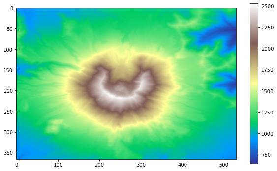

Slope

The concept of slope is simple: How much does elevation change within an area? Steep areas have lots of elevation change over a short distance while flat areas have very little. However, applying that concept to a 2D array raises the question, how do we define change within an area?

There have been many different slope algorithms created to answer that question, and each produces slightly different results. We're going to use the Horn 1981 algorithm since it is widely used (supported by GDAL, GRASS, Whitebox Tools, ESRI, etc.) but if you want to dive into the rabbit hole of slope algorithm comparisons, check out this site or this paper.

Horn's algorithm calculates slope for each pixel using the following equation, where $\frac{dz}{dx}$ is the east-west gradient of neighboring pixels and $\frac{dz}{dy}$ is the north-south gradient.

Let's break that equation down by calculating the slope of a single pixel.

One Pixel at a Time

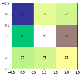
Imagine we want to calculate slope for the center pixel of a 3x3 pixel neighborhood $w$ with the following elevations:

python
Copy
import numpy as np

w = np.array([
    [52, 74, 73],
    [63, 98, 89],
    [72, 73, 75],
])

plt.imshow(w, cmap="terrain")
for (y, x), z in np.ndenumerate(w):
    plt.text(x, y, z, ha="center", va="center")

East-West Gradient

The first term in the Horn algorithm, the east-west gradient $\frac{dz}{dx}$, describes how elevation changes between the east and west side of the pixel neighborhood. To solve it, we'll break it down into the change in elevation $dz$ over the horizontal distance $dx$.

The vertical distance between pixels, $dz$, is calculated with the following equation, where the northwest pixel in the neighborhood is labeled $z_{nw}$, the southwest pixel is labeled $z_{sw}$, and so on.

There are a few things to notice in the equation above.

1. We're calculating the difference between the sum of the western and eastern pixels.
2. The directly west and east pixels, $z_{w}$ and $z_{e}$, are multiplied by 2 to increase their weight over the diagonal pixels.
3. The result is divided by 8 to normalize the value based on the input weights.

Here's $dz$ in code:

python
Copy
dz = ((w[0][0] + w[1][0] * 2 + w[2][0]) - (w[0][2] + w[1][2] * 2 + w[2][2])) / 8

The horizontal distance between pixels, $dx$, is simply the raster resolution (for this example, 30).

python
Copy
dx = 30

Now we can calculate $\frac {dz}{dx}$, the change in elevation over the $x$ dimension, by simply dividing the two terms.

python
Copy
dz_dx = dz / dx

North-South Gradient

The second term in the Horn algorithm, the north-south gradient $\frac{dz}{dy}$, describes how elevation changes between the north and south side of the pixel neighborhood. It's solution is nearly identical to the east-west gradient, after swapping in the appropriate pixels.

And in code:

python
Copy
dz = ((w[2][0] + w[2][1] * 2 + w[2][2]) - (w[0][0] + w[0][1] * 2 + w[0][2])) / 8

Assuming our image has square pixels, the distance between pixels in the north-south dimension $dy$ will be the same as $dx$.

python
Copy
dy = 30

The last step in calculating the north-south gradient is to divide the change in elevation over the $y$ dimension by the horizontal distance between cells.

python
Copy
dz_dy = dz / dy

Putting It Together

With the east-west and north-south gradients calculated, $\frac{dz}{dx}$ and $\frac{dz}{dy}$ respectiely, solving the Horn algorithm is straightforward. Just plug the two solved terms into the original equation.

python
Copy
slope_pct = np.sqrt(dz_dx ** 2 + dz_dy ** 2)

With a little more work, we can convert the percent slope into more familiar degrees of slope.

python
Copy
slope = np.arctan(slope_pct) * (180 / np.pi)
slope

18.130932944052347

For convenience, let's simplify the code above and package it into a function that will calculate the slope of a single pixel given it's 3x3 neighborhood of pixels.

python
Copy
def pixel_slope(w, resolution):
    dz_dx = ((w[0][0] + w[1][0] * 2 + w[2][0]) - (w[0][2] + w[1][2] * 2 + w[2][2])) / (8 * resolution)
    dz_dy = ((w[2][0] + w[2][1] * 2 + w[2][2]) - (w[0][0] + w[0][1] * 2 + w[0][2])) / (8 * resolution)
    
    return np.arctan(np.sqrt(dz_dx ** 2 + dz_dy ** 2)) * (180 / np.pi)

pixel_slope(w, 30)

18.130932944052347

With the fundamentals of Horn's algorithm down, the challenge now is simply to calculate it for each pixel.

Scaling Up

To calculate slope from our elevation data, we'll iterate over each row and column in the DEM, grab the 3x3 window of neighboring pixels, use the pixel_slope function to calculate the slope of the center pixel, and store the result in an empty slope array.

First, we'll create the empty array to store slope values. We'll make it two pixels smaller than the DEM in the x and y dimensions to account for the fact that edge pixels don't have the eight required neighbors.

python
Copy
slope = np.empty((dem.shape[0] - 2, dem.shape[1] - 2))
slope.shape

(364, 528)

Now we'll iterate over rows and columns (dropping one pixel from each side to account for edges) and calculate slope for each neighborhood of pixels.

python
Copy
for row in range(1, dem.shape[0] - 1):
    for col in range(1, dem.shape[1] - 1):        
        w = dem[row-1:row+2, col-1:col+2]
        slope[row-1][col-1] = pixel_slope(w, 30)

Finally, let's see what our slope map looks like, with flat areas in blue and steep areas in red.

python
Copy
plt.figure(figsize=(10, 6))
plt.imshow(slope, cmap="RdBu_r")
plt.colorbar()

<matplotlib.colorbar.Colorbar at 0x7f7e6f70d4f0>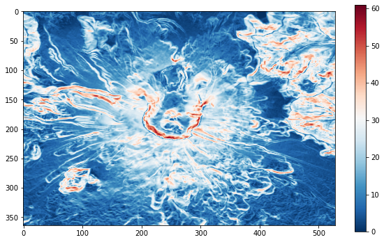

Aspect

Aspect is closely related to slope, describing orientation rather than steepness. Since we've already implemented the Horn slope algorithm, we'll use that for calculating aspect as well, with the following equation.

The east-west and north-south gradients, $\frac{dz}{dx}$ and $\frac{dz}{dy}$ respectiely, are calculated identically to slope. The only difference is that instead of taking the square root of their sum to get the overall slope, we use the arctangent to calculate the angle between them.

Here's that equation in code, plus conversion to degrees and rescaling to compass bearings:

python
Copy
def pixel_aspect(w, resolution):
    """Calculate the aspect of a pixel in degrees given its 3x3 neighborhood `w` and cell resolution."""
    dz_dx = ((w[0][0] + w[1][0] * 2 + w[2][0]) - (w[0][2] + w[1][2] * 2 + w[2][2])) / (8 * resolution)
    dz_dy = ((w[2][0] + w[2][1] * 2 + w[2][2]) - (w[0][0] + w[0][1] * 2 + w[0][2])) / (8 * resolution)
    
    aspect = np.arctan2(dz_dy, dz_dx) * (180 / np.pi)
    # Convert to compass bearings 0 - 360
    aspect = 450 - aspect if aspect > 90 else 90 - aspect

    return aspect
    
pixel_aspect(w, 30)

184.12761236173162

We calculate aspect for each pixel the same way we did slope, by iteratively filling an empty 2D array with aspects calculated from each pixel's 3x3 neighborhood.

python
Copy
aspect = np.empty((dem.shape[0] - 2, dem.shape[1] - 2))

for row in range(1, dem.shape[0] - 1):
    for col in range(1, dem.shape[1] - 1):        
        w = dem[row-1:row+2, col-1:col+2]
        aspect[row-1][col-1] = pixel_aspect(w, 30)

plt.figure(figsize=(10, 6))
plt.imshow(aspect, cmap="magma")
plt.colorbar()

<matplotlib.colorbar.Colorbar at 0x7f7e6f650ac0>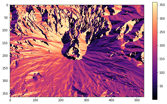

Hillshading

With slope and aspect calculated, generating hillshading to visualize the terrain is simple.

The formula to calculate hillshading is below, with all units in radians. The zenith and azimuth parameters describe the position of the simulated light source, and can be tuned to adjust the hillshading effect.

Here's that equation in code, using the slope and aspect arrays we calculated earlier.

python
Copy
azimuth = 315
altitude = 45

# Convert solar altitude to zenith and convert everything to radians
zenith_rad = 90 - altitude * np.pi / 180
azimuth_rad = azimuth * np.pi / 180
slope_rad = slope * np.pi / 180
aspect_rad = aspect * np.pi / 180

# Calculate hillshade and scale to 8-bit
hs = 255 * (np.cos(zenith_rad) * np.cos(slope_rad) + np.sin(zenith_rad) * np.sin(slope_rad) * np.cos(azimuth_rad - aspect_rad))
# Clip out-of-bounds values
hs = np.clip(hs, 0, 255)

plt.figure(figsize=(10, 6))
plt.imshow(hs, cmap="Greys_r")

<matplotlib.image.AxesImage at 0x7f7e7d0339d0>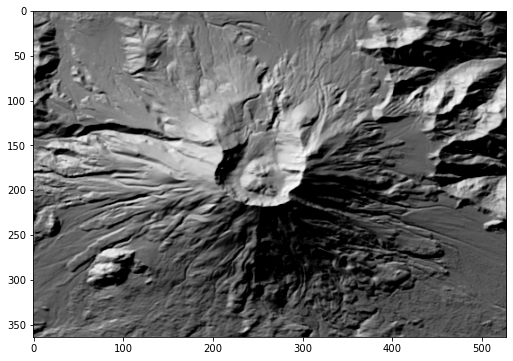

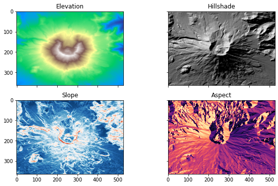
Wrapping Up

Now that we know how to implement terrain algorithms from scratch, the next step is to uninstall QGIS, WhiteboxTools, GDAL, and any other geospatial tools we no longer need!

Okay, probably not. There are faster and more convenient ways to generate terrain data than rolling your own implementations, but getting a glimpse at the underlying algorithms does provide some interesting insights into how they work.

python
Copy
fig, axs = plt.subplots(2, 2, sharex=True, sharey=True, figsize=(10, 6))

axs[0, 0].set_title("Elevation")
axs[0, 0].imshow(dem, cmap="terrain")

axs[0, 1].set_title("Hillshade")
axs[0, 1].imshow(hs, cmap="Greys_r")

axs[1, 0].set_title("Slope")
axs[1, 0].imshow(slope, cmap="RdBu_r")

axs[1, 1].set_title("Aspect")
axs[1, 1].imshow(aspect, cmap="magma")

<matplotlib.image.AxesImage at 0x7f7e6f560d90>